决策树的本质

1. 损失函数 -- 总信息熵

因为要把一个东西转向为一个确定的分类结果,所以信息熵应该是最低的.

2. 梯度 -- 信息增益

3. 决策树 - 梯度下降路径

4. 非参数模型

二分类信息熵

import numpy as np
from matplotlib import pyplot as plt

# 信息熵
# 这里定义的信息熵是总体样本所含信息熵.
def entropy(p):
    return -p*np.log2(p)-(1-p)*np.log2(1-p)

plot_x = np.linspace(0.001,0.999,100)
plt.plot(plot_x,entropy(plot_x))
plt.show()
# 在图中p=0.5时不确定性程度最高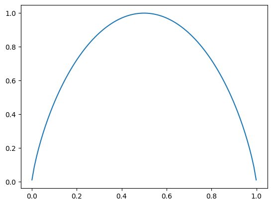

from sklearn.datasets import load_iris
iris = load_iris()
X = iris.data[:,:2]
y = iris.target
X[:5]

运行结果

 array([[5.1, 3.5], [4.9, 3. ], [4.7, 3.2], [4.6, 3.1], [5. , 3.6]]) 

plt.scatter(X[:,0],X[:,1],c=y)
plt.show()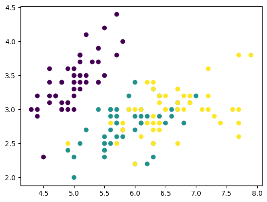

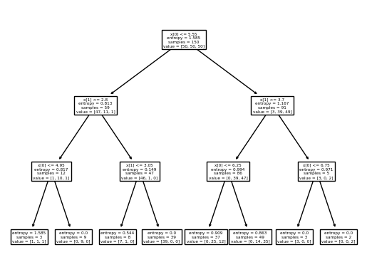
from sklearn.tree  import DecisionTreeClassifier

clf = DecisionTreeClassifier(max_depth=3,criterion='entropy')
clf.fit(X,y)

运行结果

 DecisionTreeClassifier(criterion='entropy', max_depth=3) 

clf.score(X,y)

运行结果

 0.8066666666666666 

from sklearn.tree import plot_tree
plot_tree(clf)

运行结果

 [Text(0.5, 0.875, 'x[0] <= 5.55\nentropy = 1.585\nsamples = 150\nvalue = [50, 50, 50]'), Text(0.25, 0.625, 'x[1] <= 2.8\nentropy = 0.813\nsamples = 59\nvalue = [47, 11, 1]'), Text(0.125, 0.375, 'x[0] <= 4.95\nentropy = 0.817\nsamples = 12\nvalue = [1, 10, 1]'), Text(0.0625, 0.125, 'entropy = 1.585\nsamples = 3\nvalue = [1, 1, 1]'), Text(0.1875, 0.125, 'entropy = 0.0\nsamples = 9\nvalue = [0, 9, 0]'), Text(0.375, 0.375, 'x[1] <= 3.05\nentropy = 0.149\nsamples = 47\nvalue = [46, 1, 0]'), Text(0.3125, 0.125, 'entropy = 0.544\nsamples = 8\nvalue = [7, 1, 0]'), Text(0.4375, 0.125, 'entropy = 0.0\nsamples = 39\nvalue = [39, 0, 0]'), Text(0.75, 0.625, 'x[1] <= 3.7\nentropy = 1.167\nsamples = 91\nvalue = [3, 39, 49]'), Text(0.625, 0.375, 'x[0] <= 6.25\nentropy = 0.994\nsamples = 86\nvalue = [0, 39, 47]'), Text(0.5625, 0.125, 'entropy = 0.909\nsamples = 37\nvalue = [0, 25, 12]'), Text(0.6875, 0.125, 'entropy = 0.863\nsamples = 49\nvalue = [0, 14, 35]'), Text(0.875, 0.375, 'x[0] <= 6.75\nentropy = 0.971\nsamples = 5\nvalue = [3, 0, 2]'), Text(0.8125, 0.125, 'entropy = 0.0\nsamples = 3\nvalue = [3, 0, 0]'), Text(0.9375, 0.125, 'entropy = 0.0\nsamples = 2\nvalue = [0, 0, 2]')] 

### 寻找最优化分条件

from collections import Counter
Counter(y)

运行结果

 Counter({0: 50, 1: 50, 2: 50}) 

def calc_entropy(y):
    counter =Counter(y)
    sum_entropy = 0
    for num in counter:
        p = counter[num]/len(y)
        # sum_entropy += entropy(p)
        sum_entropy += (-p*np.log2(p))
    return sum_entropy

calc_entropy(y)

运行结果

 1.584962500721156 

# 分割样本函数
def split_dataset(x,y,dim,value):
    index_left = x[:,dim]<=value
    index_right = x[:,dim]>value
    return x[index_left],y[index_left],x[index_right],y[index_right]

def find_best_split(X, y):
    best_dim = -1
    best_val = -1
    best_entropy = np.inf
    best_entropy_left,best_entropy_right = -1,-1
    # 遍历列数
    for dim in range(X.shape[1]):
        sorted_idx = np.argsort(X[:, dim])
        # 便利所有行数,即遍历所有分裂点
        # 因为后面有一个i+1,所以需要减去1
        for i in range(X.shape[0]-1):
            # 获取当前和下一个的值
            value_left,value_right = X[sorted_idx[i], dim],X[sorted_idx[i+1], dim]
            val = (value_left + value_right) / 2
            x_left,y_left,x_right,y_right = split_dataset(X, y, dim, val)
            # 计算熵值
            entropy_left,entropy_right = calc_entropy(y_left),calc_entropy(y_right)
            entropy = entropy_left*len(y_left)/len(y) + entropy_right*len(y_right)/len(y)
            # 记录最好的划分
            if entropy < best_entropy:
                best_dim = dim
                best_val = val
                best_entropy = entropy
                best_entropy_left,best_entropy_right = entropy_left,entropy_right
    return best_dim,best_val,best_entropy,best_entropy_left,best_entropy_right

find_best_split(X,y)
# 在左子树右子树可以继续调用find_best_split函数

运行结果

 (0, 5.5, 1.0277298129142294, 0.8128223064150747, 1.167065448996099)