import numpy as np
from matplotlib import pyplot as plt

x = np.random.uniform(-4,2,100)
y=2*x**2+4*x+3+np.random.randn(100)
X = x.reshape(-1,1)

plt.scatter(x,y)
plt.show()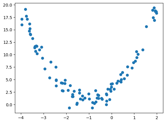

from sklearn.linear_model import LinearRegression
lin_reg = LinearRegression()
lin_reg.fit(x.reshape(-1,1),y)

运行结果

 LinearRegression() 

y_predict = lin_reg.predict(X)
plt.scatter(X, y, color='red')
plt.plot(X, y_predict, label='data')
plt.show()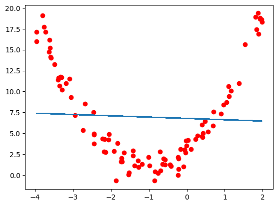

### 多项式回归

X[:5]

运行结果

 array([[-2.73686204], [-3.75805097], [-1.53060284], [-3.61514055], [-1.41108905]]) 

添加一个二次项$x^2$，并将其加入到模型中：

X_new = np.hstack([X,X**2])
# horizontal 水平 合并

X_new[:5]

运行结果

 array([[-2.73686204, 7.49041384], [-3.75805097, 14.12294708], [-1.53060284, 2.34274506], [-3.61514055, 13.06924117], [-1.41108905, 1.9911723 ]]) 

ln_new =LinearRegression()
ln_new.fit(X_new,y)
y_pred = ln_new.predict(X_new)
plt.scatter(X, y, color='red')
# 这里因为matplotlib是从左到右依次连线，所以需要先排序
plt.plot(np.sort(x), y_pred[np.argsort(x)], label='data')
plt.show()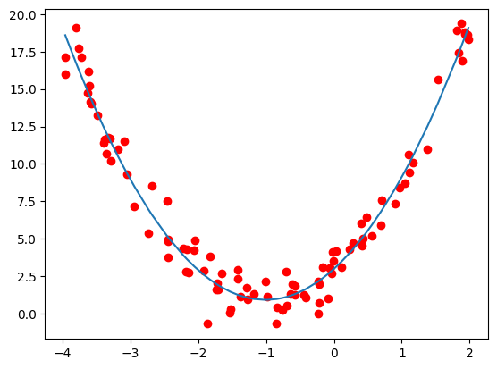

ln_new.coef_,ln_new.intercept_

运行结果

 (array([4.10591861, 2.03437628]), 2.9743198164240843) 

ln_new.score(X_new,y)

运行结果

 0.9672452031085343 

使用PolynomialFeatures构造高次多项式特征

from sklearn.preprocessing import PolynomialFeatures

poly_features = PolynomialFeatures(degree=2)
X_poly = poly_features.fit_transform(x.reshape(-1,1))
X_poly[:5]

运行结果

 array([[ 1. , -2.73686204, 7.49041384], [ 1. , -3.75805097, 14.12294708], [ 1. , -1.53060284, 2.34274506], [ 1. , -3.61514055, 13.06924117], [ 1. , -1.41108905, 1.9911723 ]])